Edit (09/07/17): Sorry for the long quiet interval. It was (partly) due to the fact that I took some time to refine some the code and the arguments in this and the previous post and put it into a paper, of which there is a preprint available as of today: http://arxiv.org/abs/1709.02341 🙂
Edit (11/14/18): A thoroughly corrected (beware of typos beyond this point!) and extended version of the material in this and the previous post was published in Biological Cybernetics. You can find a copy of the author’s accepted manuscript here.
In the last post I tried to summarise the rationale behind the free energy principle and the resulting active inference dynamics. I will assume you read this post and have a rough idea about the free energy principle for action and perception. Now I want to get concrete and introduce you to what I call a “Deep Active Inference” agent. While I tried to minimize formalism in the last post, I’m sorry that it will get quite technical now. But I will try and be very specific in this post, to allow people to implement their own versions of this type of agent. You can find a reference implementation here.
The Environment
Our agent will live in a discrete version of the mountaincar world. It will start at the bottom 

Our agent is a small car on this landscape, whose true, physical state 


The dynamics are given by a set of update equations, which can be summarised symbolically by
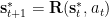
Here the next physical state depends on the current physical state and the action state 

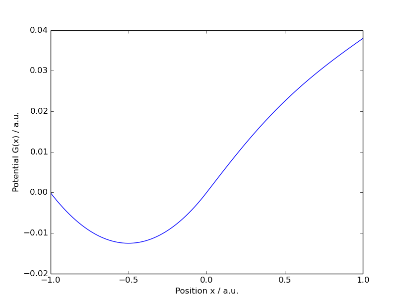
This equation can be decomposed into a set of equations. First we have the downhill force 


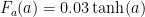
The agent’s motor can generate a force 

Finally, we have a laminar friction force 

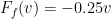
Combined, this yields the total force acting on the agent:

We use this force to update the velocity:

and then update the position:
The initial state of our agent is resting at the bottom of the landscape, i.e.

The goal of our agent will be to reach and stay at 
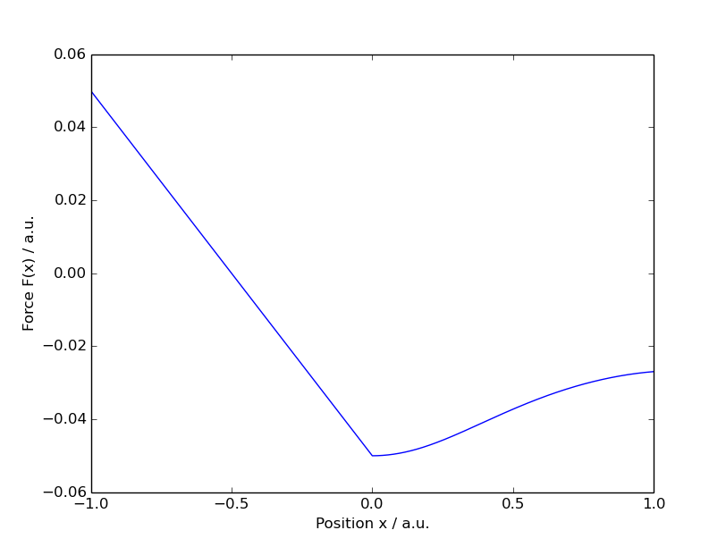

we notice that the landscape gets very steep at 
As the action force generated by the motor is limited to the interval 


The Agent
Sensory Inputs
Our agent has a noisy sense 

To show that the agent can indeed learn a complex, nonlinear, generative model of its sensory input, we add another sensory channel with a nonlinear, non-bijective transformation of

One could use this sensory channel as a “reward” channel, as it encodes the agent’s distance to what we will later define as its “goal position”, 
Note that the agent has no direct measurement of its current velocity
To see if the agent understands its own actions, we also give it a proprioceptive sensory channel, allowing it to feel its current action state

Note that having a concrete sense of its action state is *not* necessary for an active inference agent to successfully control its environment. E.g. the reflex arcs that we use to increase the likelihood of our sensory inputs, given our generative model of the world, feature their own, closed loop neural dynamics at the level of the spinal cord. So we do not (and do not have to) have direct access to the “action states” of our muscles, when we just lift our arm by expecting it to lift. However, adding this channel will allow us later to directly sample the agents proprioceptive sensations from its generative model, to check if it understands its own action on the environment.
The Agent’s Generative Model of the Environment
First, the agent has a prior over the hidden states 

with the initial state, before it has encountered any observations, 
This factorisation means that the next state 


We use 
Similarly, the likelihood functions for each of the three observables also factorise
![p_\theta(o_{x,1}, ..., o_{x,T},o_{h,1}, ..., o_{h,T},o_{a,1}, ..., o_{a,t}|\mathbf{s}_1, ...., \mathbf{s}_T) \\ \vphantom{ \left[ \left< -\ln p_\theta^{x,l}\right>_{q_\theta} \right] }\qquad= \prod_{t=0}^T p_\theta (o_{x,t} | \mathbf{s}_t) \prod_{t=0}^T p_\theta (o_{h,t} | \mathbf{s}_t) \prod_{t=0}^T p_\theta (o_{a,t} | \mathbf{s}_t)](https://s0.wp.com/latex.php?latex=p_%5Ctheta%28o_%7Bx%2C1%7D%2C+...%2C+o_%7Bx%2CT%7D%2Co_%7Bh%2C1%7D%2C+...%2C+o_%7Bh%2CT%7D%2Co_%7Ba%2C1%7D%2C+...%2C+o_%7Ba%2Ct%7D%7C%5Cmathbf%7Bs%7D_1%2C%C2%A0....%2C+%5Cmathbf%7Bs%7D_T%29+%5C%5C++%5Cvphantom%7B%C2%A0%5Cleft%5B+%5Cleft%3C+-%5Cln+p_%5Ctheta%5E%7Bx%2Cl%7D%5Cright%3E_%7Bq_%5Ctheta%7D+%5Cright%5D+%C2%A0%7D%5Cqquad%3D%C2%A0%5Cprod_%7Bt%3D0%7D%5ET+p_%5Ctheta+%28o_%7Bx%2Ct%7D+%7C+%5Cmathbf%7Bs%7D_t%29+%5Cprod_%7Bt%3D0%7D%5ET+p_%5Ctheta+%28o_%7Bh%2Ct%7D+%7C+%5Cmathbf%7Bs%7D_t%29+%5Cprod_%7Bt%3D0%7D%5ET+p_%5Ctheta+%28o_%7Ba%2Ct%7D+%7C+%5Cmathbf%7Bs%7D_t%29++&bg=ffffff&fg=000000&s=0&c=20201002)
So the likelihood of each observable 


Sampling from the Generative Model
Once the agent has acquired a generative model of its sensory inputs, by optimising the parameters
- Evaluate
using the state
sampled at the previous iteration.
- Draw a single sample
- Use this sample to evaluate the likelihoods
- Sample a single observation
- Carry over

The fact that we will sample many processes in parallel will allow us to get a good approximation, although we only sample once per individual process and per timestep.
Variational Density
Following Kingma & Welling/Rezende, Mohamed & Wierstra we do not explicitly represent the sufficient statistics of the variational posterior at every time step. This would require an additional, costly optimisation of these variational parameters at each individual time step. Instead we use an inference network, which approximates the dependency of the variational posterior on the previous state and the current sensory input and which is parameterised by time-invariant parameters. This allows us to learn these parameters together with the parameters of the generative model and the action function (c.f. below) and also allows for very fast inference later on. We use the following factorisation for this approximation of the variational density (approximate posterior) on the states 
![q_\theta(\mathbf{s}_1, ..., \mathbf{s}_T | o_{x,1}, ..., o_{x,T},o_{h,1}, ..., o_{h,T}, o_{a,1}, ..., o_{a,T}) \\ \vphantom{ \left[ \left< -\ln p_\theta^{x,l}\right>_{q_\theta} \right] }\qquad = \prod_{t=1}^T q_\theta(\mathbf{s}_t | \mathbf{s}_{t-1}, o_{x,t}, o_{h,t}, o_{a,t})](https://s0.wp.com/latex.php?latex=q_%5Ctheta%28%5Cmathbf%7Bs%7D_1%2C+...%2C+%5Cmathbf%7Bs%7D_T+%7C%C2%A0o_%7Bx%2C1%7D%2C+...%2C+o_%7Bx%2CT%7D%2Co_%7Bh%2C1%7D%2C+...%2C+o_%7Bh%2CT%7D%2C+o_%7Ba%2C1%7D%2C+...%2C+o_%7Ba%2CT%7D%29+%5C%5C++%5Cvphantom%7B%C2%A0%5Cleft%5B+%5Cleft%3C+-%5Cln+p_%5Ctheta%5E%7Bx%2Cl%7D%5Cright%3E_%7Bq_%5Ctheta%7D+%5Cright%5D+%C2%A0%7D%5Cqquad+%3D%C2%A0%5Cprod_%7Bt%3D1%7D%5ET+q_%5Ctheta%28%5Cmathbf%7Bs%7D_t+%7C+%5Cmathbf%7Bs%7D_%7Bt-1%7D%2C+o_%7Bx%2Ct%7D%2C+o_%7Bh%2Ct%7D%2C+o_%7Ba%2Ct%7D%29++&bg=ffffff&fg=000000&s=0&c=20201002)
and we again use diagonal Gaussians
![q_\theta(\mathbf{s}_t | \mathbf{s}_{t-1}, o_{x,t}, o_{h,t}, o_{a,t}) \\ \vphantom{ \left[ \left< -\ln p_\theta^{x,l}\right>_{q_\theta} \right] }\qquad = \mathrm{N}(\mathbf{s}_t; \boldsymbol{\mu}^q_\theta(\mathbf{s}_{t-1}, o_{x,t}, o_{h,t}, o_{a,t}), \boldsymbol{\sigma}^q_\theta(\mathbf{s}_{t-1}, o_{x,t}, o_{h,t}, o_{a,t}))](https://s0.wp.com/latex.php?latex=q_%5Ctheta%28%5Cmathbf%7Bs%7D_t+%7C+%5Cmathbf%7Bs%7D_%7Bt-1%7D%2C+o_%7Bx%2Ct%7D%2C+o_%7Bh%2Ct%7D%2C+o_%7Ba%2Ct%7D%29+%5C%5C++%5Cvphantom%7B%C2%A0%5Cleft%5B+%5Cleft%3C+-%5Cln+p_%5Ctheta%5E%7Bx%2Cl%7D%5Cright%3E_%7Bq_%5Ctheta%7D+%5Cright%5D+%C2%A0%7D%5Cqquad+%3D+%5Cmathrm%7BN%7D%28%5Cmathbf%7Bs%7D_t%3B+%5Cboldsymbol%7B%5Cmu%7D%5Eq_%5Ctheta%28%5Cmathbf%7Bs%7D_%7Bt-1%7D%2C+o_%7Bx%2Ct%7D%2C+o_%7Bh%2Ct%7D%2C+o_%7Ba%2Ct%7D%29%2C+%5Cboldsymbol%7B%5Csigma%7D%5Eq_%5Ctheta%28%5Cmathbf%7Bs%7D_%7Bt-1%7D%2C+o_%7Bx%2Ct%7D%2C+o_%7Bh%2Ct%7D%2C+o_%7Ba%2Ct%7D%29%29++&bg=ffffff&fg=000000&s=0&c=20201002)
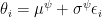
Action States
In general, the action state 

whose parameters we include, together with the parameters of the generative model and the variational density, to the set of parameters
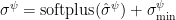
Again we use a diagonal Gaussian form and neural networks to calculate the means and standard deviations:

We now can just optimise the time-invariant parameters
The approximation of both the sufficient statistics of the variational density
However, in this very concrete case it turned out, that it is enough to just use two single layer networks to calculate the mean and standard deviation of the action state
Graphical Model
All in all, the causal structure of our model looks like this:
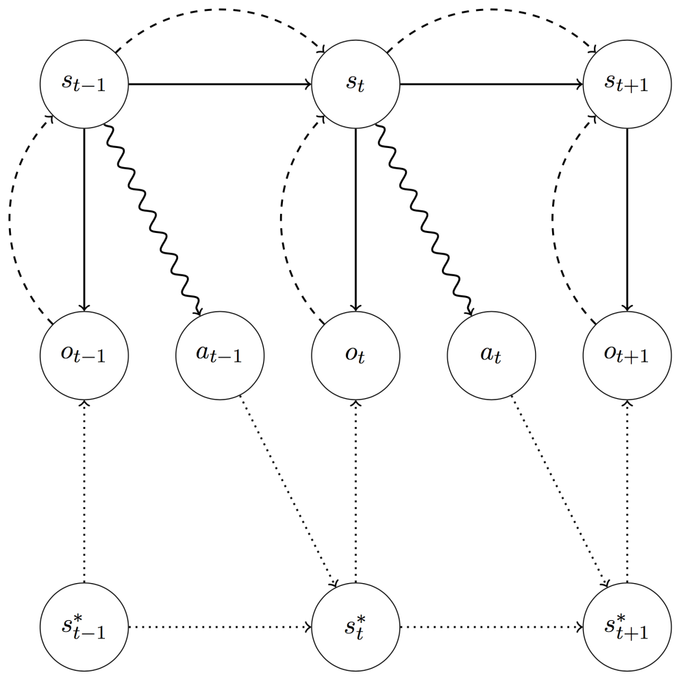
Here the solid lines correspond to the factors of the agent’s generative model, 


The Free Energy Objective
Now we have everything that we need to put our objective function together. We use the following form of the variational free energy bound (which I discussed in the previous post):
![F(o, \theta) = \left< - \ln p_\theta(o_{x,1}, ..., o_{x,T},o_{h,1}, ..., o_{h,T},o_{a,1}, ..., o_{a,t}|\mathbf{s}_1, ...., \mathbf{s}_T) \right>_q \\ \vphantom{ \left[ \left< -\ln p_\theta^{x,l}\right>_{q_\theta} \right] }\qquad\qquad\qquad + D_{KL}(q_\theta(\mathbf{s}_1, ..., \mathbf{s}_T | o_{x,1}, ..., o_{x,T},o_{h,1}, ..., o_{h,T}, o_{a,1}, ..., o_{a,T}) || p_\theta(\mathbf{s}_1, \mathbf{s}_2, ..., \mathbf{s}_T) )](https://s0.wp.com/latex.php?latex=F%28o%2C+%5Ctheta%29+%3D+%5Cleft%3C+-+%5Cln+p_%5Ctheta%28o_%7Bx%2C1%7D%2C+...%2C+o_%7Bx%2CT%7D%2Co_%7Bh%2C1%7D%2C+...%2C+o_%7Bh%2CT%7D%2Co_%7Ba%2C1%7D%2C+...%2C+o_%7Ba%2Ct%7D%7C%5Cmathbf%7Bs%7D_1%2C%C2%A0....%2C+%5Cmathbf%7Bs%7D_T%29+%5Cright%3E_q+%5C%5C++%5Cvphantom%7B%C2%A0%5Cleft%5B+%5Cleft%3C+-%5Cln+p_%5Ctheta%5E%7Bx%2Cl%7D%5Cright%3E_%7Bq_%5Ctheta%7D+%5Cright%5D+%C2%A0%7D%5Cqquad%5Cqquad%5Cqquad+%2B+D_%7BKL%7D%28q_%5Ctheta%28%5Cmathbf%7Bs%7D_1%2C+...%2C+%5Cmathbf%7Bs%7D_T+%7C%C2%A0o_%7Bx%2C1%7D%2C+...%2C+o_%7Bx%2CT%7D%2Co_%7Bh%2C1%7D%2C+...%2C+o_%7Bh%2CT%7D%2C+o_%7Ba%2C1%7D%2C+...%2C+o_%7Ba%2CT%7D%29+%7C%7C+p_%5Ctheta%28%5Cmathbf%7Bs%7D_1%2C+%5Cmathbf%7Bs%7D_2%2C+...%2C+%5Cmathbf%7Bs%7D_T%29+%29++&bg=ffffff&fg=000000&s=0&c=20201002)
where 

Using the above factorisation, the free energy becomes:
![F(o, \theta) = \sum_{t=1}^T \left[ \left< -\ln p_\theta(o_{x,t}|\mathbf{s}_t) -\ln p_\theta(o_{h,t}|\mathbf{s}_t) -\ln p_\theta(o_{a,t}|\mathbf{s}_t) \right>_{q_\theta(\mathbf{s}_t|\mathbf{s}_{t-1},o_{x,t},o_{a,t},o_{h,t})} \right. \\ \phantom{.}\qquad\qquad\qquad\qquad + \left. \vphantom{ \left< -\ln p_\theta^{x,l}\right>_{q_\theta} } D_{KL} (q_\theta(\mathbf{s}_t|\mathbf{s}_{t-1},o_{x,t},o_{a,t},o_{h,t}) ||p_\theta ( \mathbf{s}_t | \mathbf{s}_{t-1})) \right]](https://s0.wp.com/latex.php?latex=F%28o%2C+%5Ctheta%29+%3D+%5Csum_%7Bt%3D1%7D%5ET+%5Cleft%5B+%5Cleft%3C+-%5Cln+p_%5Ctheta%28o_%7Bx%2Ct%7D%7C%5Cmathbf%7Bs%7D_t%29%C2%A0-%5Cln+p_%5Ctheta%28o_%7Bh%2Ct%7D%7C%5Cmathbf%7Bs%7D_t%29+-%5Cln+p_%5Ctheta%28o_%7Ba%2Ct%7D%7C%5Cmathbf%7Bs%7D_t%29+%5Cright%3E_%7Bq_%5Ctheta%28%5Cmathbf%7Bs%7D_t%7C%5Cmathbf%7Bs%7D_%7Bt-1%7D%2Co_%7Bx%2Ct%7D%2Co_%7Ba%2Ct%7D%2Co_%7Bh%2Ct%7D%29%7D+%5Cright.+%5C%5C++%5Cphantom%7B.%7D%5Cqquad%5Cqquad%5Cqquad%5Cqquad+%2B+%5Cleft.+%5Cvphantom%7B%C2%A0%5Cleft%3C+-%5Cln+p_%5Ctheta%5E%7Bx%2Cl%7D%5Cright%3E_%7Bq_%5Ctheta%7D+%7D+D_%7BKL%7D+%28q_%5Ctheta%28%5Cmathbf%7Bs%7D_t%7C%5Cmathbf%7Bs%7D_%7Bt-1%7D%2Co_%7Bx%2Ct%7D%2Co_%7Ba%2Ct%7D%2Co_%7Bh%2Ct%7D%29+%7C%7Cp_%5Ctheta+%C2%A0%28+%5Cmathbf%7Bs%7D_t+%7C+%5Cmathbf%7Bs%7D_%7Bt-1%7D%29%29+%5Cright%5D++&bg=ffffff&fg=000000&s=0&c=20201002)
Ooookay, but how do we evaluate this humongous expression? The idea is that we simulate several thousand processes in parallel, which allows us to approximate the variational density
- For each timestep, we first calculate the means and standard deviations
of
, using the sampled state
from the previous timestep, where
, and the current observations.
- Then we draw a single sample of
, approximating the expectation over
- We calculate the means and standard deviations
of the prior
using the sample
- To generate the observations for the next timestep, we draw a single sample from
, using our sample of
(i.e. the simulated world), to generate the next state of the world and the resulting observations
. Initially we use
.
- We can now evaluate the next timestep, using the new observations and the sampled state

As stated above, the fact that we will be running a lot of processes in parallel allows us to resort to this simple sampling scheme for the individual processes.
The minimisation of the free energy with respect to the parameters 


![\begin{array}{rcl} F(o, \theta) & = & <- \ln p_\theta(o|\mathbf{s})>_{q_\theta(\mathbf{s}|o)} \vphantom{ \left[ \left< -\ln p_\theta^{x,l}\right>_{q_\theta} \right] }+ D_{KL}(q_\theta(\mathbf{s}|o)||p_\theta(\mathbf{s})) \\ & =\vphantom{ \left[ \left< -\ln p_\theta^{x,l}\right>_{q_\theta} \right] } & - \ln p_\theta(o) + D_{KL}(q_\theta(\mathbf{s}|o)||p_\theta(\mathbf{s}|o)) \end{array}](https://s0.wp.com/latex.php?latex=%5Cbegin%7Barray%7D%7Brcl%7D++F%28o%2C+%5Ctheta%29+%26+%3D+%26+%3C-+%5Cln+p_%5Ctheta%28o%7C%5Cmathbf%7Bs%7D%29%3E_%7Bq_%5Ctheta%28%5Cmathbf%7Bs%7D%7Co%29%7D+%5Cvphantom%7B%C2%A0%5Cleft%5B+%5Cleft%3C+-%5Cln+p_%5Ctheta%5E%7Bx%2Cl%7D%5Cright%3E_%7Bq_%5Ctheta%7D+%5Cright%5D+%C2%A0%7D%2B+D_%7BKL%7D%28q_%5Ctheta%28%5Cmathbf%7Bs%7D%7Co%29%7C%7Cp_%5Ctheta%28%5Cmathbf%7Bs%7D%29%29+%5C%5C++%26+%3D%5Cvphantom%7B%C2%A0%5Cleft%5B+%5Cleft%3C+-%5Cln+p_%5Ctheta%5E%7Bx%2Cl%7D%5Cright%3E_%7Bq_%5Ctheta%7D+%5Cright%5D+%C2%A0%7D+%26%C2%A0-+%5Cln+p_%5Ctheta%28o%29+%2B+D_%7BKL%7D%28q_%5Ctheta%28%5Cmathbf%7Bs%7D%7Co%29%7C%7Cp_%5Ctheta%28%5Cmathbf%7Bs%7D%7Co%29%29++%5Cend%7Barray%7D++&bg=ffffff&fg=000000&s=0&c=20201002)
Additionally, the parameters of the action function will be optimised, so that the agent seeks out expected states under its own model of the world, minimizing 
Optimising its generative model of the world gives the agent a sense of epistemic value. I.e. it will not only seek out the states, which it expects, but it will also try to improve its general understanding of the world. This is very similar to (but in my opinion more natural than) recent work on artificial curiosity. However, in contrast to this work, our agent is not only interested in those environmental dynamics which it can directly influence by its own action, but also tries to learn the statistics of its environment which are beyond its control.
Goal Directed Behavior
If we just propagate and optimise our agent as it is now, it will look for a stable equilibrium with its environment and settle there. However, to be practically applicable to real-life problems, we have to instil some concrete goals in our agent. We can achieve this by defining states that it will expect to be in. Then the action states will try to fulfil these expectations.
In this concrete case, we want to propagate the agent for 30 timesteps and want it to be at

This can be seen as a homeostatic, i.e. vitally important, state parameter. E.g. the CO₂ concentration in our blood is extremely important and tightly controlled, as opposed to the possible brightness perceived at the individual receptors of our retina, which can vary by orders of magnitude. Though we might not directly change our behavior depending on visual stimuli, a slight increase in the CO₂ concentration of our blood and the concurring decrease in the pH will trigger chemoreceptors in the carotid and aortic bodies, which in turn will increase the activity of the respiratory centers in the medulla oblongata and the pons, leading to a fast and strong increase in ventilation, which might be accompanied by a subjective feeling of dyspnoea or respiratory distress. These hard-wired connection between vitally important body parameters and direct changes in perception and action might be very similar to our approach to encode the goal-relevant states explicitly.
But besides explicitly encoding relevant environmental parameters in the hidden states of the agent’s latent model, we also have to specify the corresponding prior expectations (such as explicit boundaries for the pH of our blood). We do this by explicitly setting the prior over the first dimension of the state vector for 

While this kind of hard-coded inference dynamics and expectations might be fixed for individual agents of a class (i.e. species) within their lifetimes, these mappings can be optimised on a longer timescale over populations of agents by evolution. In fact, evolution might be seen as a very similar learning process, only on different spatial and temporal scales (c.f. the post of Marc Harper on John Baez’s Blog, and this talk by John Baez).
Optimization
Without action, the model and the objective would be very similar to the objective functions of Rezende, Mohamed & Wierstra, Kingma & Welling, and Chung & al and we could just sample a lot of random processes and do a gradient descent on the estimated free energy with respect to the parameters
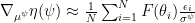
Evolution Strategies
Luckily, it was recently shown that evolution strategies allow for efficient optimisation of non-differentiable objective functions 
Instead of searching for a single optimal parameter set 


Now we can calculate the gradient of 

Using again a diagonal Gaussian for 
Following the discussion at Ferenc Huszár’s Blog, we will also optimize the standard deviations of our population density, using the following gradients (Try also to derive this on your own!):
Drawing samples 


and
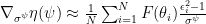
Actually, for reasons of stability we are not optimising 
with 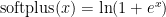


Now we have everything: A model of the world, the agent, an objective function which we can evaluate and which has gradients that we can optimise. The final step is to run your optimisation method of choice (mine is ADAM) with the gradient estimates for the means and standard-derivations of our population density and watch!
Note that we do not need any tricks like batch-normalization for our method to converge and that it can run on a single NVIDIA GPU (I tested it on the first generation Titan from 2013), using about 3GB of graphics memory.
Results (Wait? It really worked?)
So let’s look at the convergence of a simple agent with 
It quickly converges from its random starting parameters to a plateau, on which it tries to directly climb the hill and gets stuck at the steep slope. However, after a while (about 10,000 updates of the population density) it discovers, that it can get higher by first moving in the opposite direction, thereby gaining some momentum, which it can use to overcome the steep parts of the slope:
 ), it can reach a higher position than by directly going upwards. Shown are the agent’s proprioception (upper left), its sense of position (upper right), its nonlinearly transformed sensory channel
  (lower left) and its “homeostatic” hidden state
  (lower right).
This sudden, rapid decline in the free energy might (okay, I am overinterpreting, but try and stop me…) be our agents first (and in this environment only) “AHA”-moment.
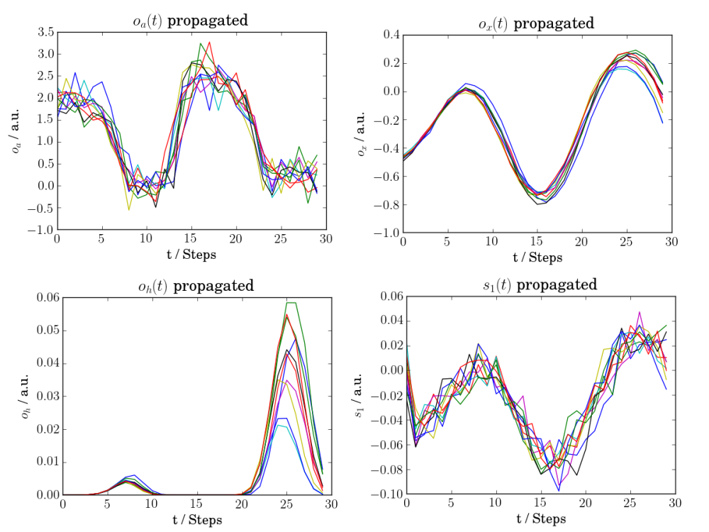
After about 50 000 iterations our agent’s trajectory looks very efficient: It takes a short left swing, to gain just the required momentum, and then it directly swings up to its target position
 (upper left). The resulting trajectory (shown in terms of , upper right) first leads uphill to the left, away from the target position, to gain momentum and overcome the steep slope at
  . The nonlinearly modified sensory channel is shown on the lower left and the “homeostatic” hidden state on the lower right.
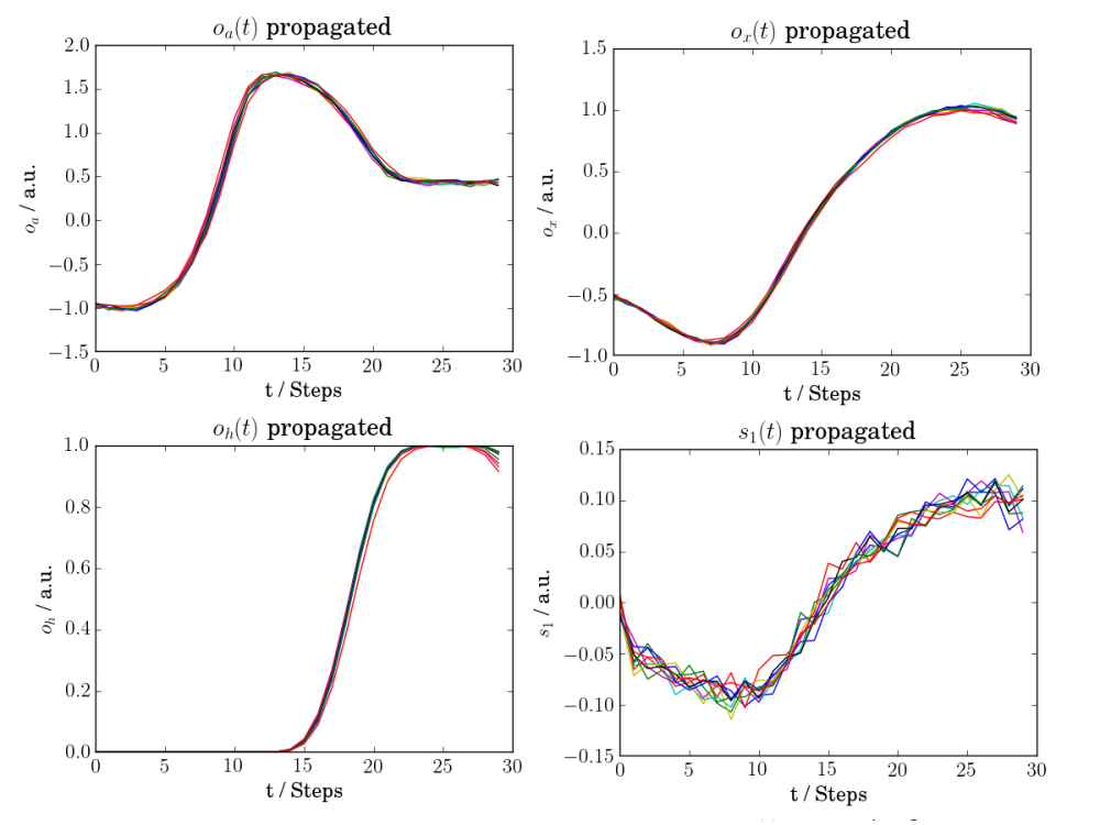
Also, our agent now has developed quite some understanding of its environment. We can compare the above image, which was generated by actually propagating the agent in its environment, with the following one, which was generated just by sampling from the agents generative model of its environment:
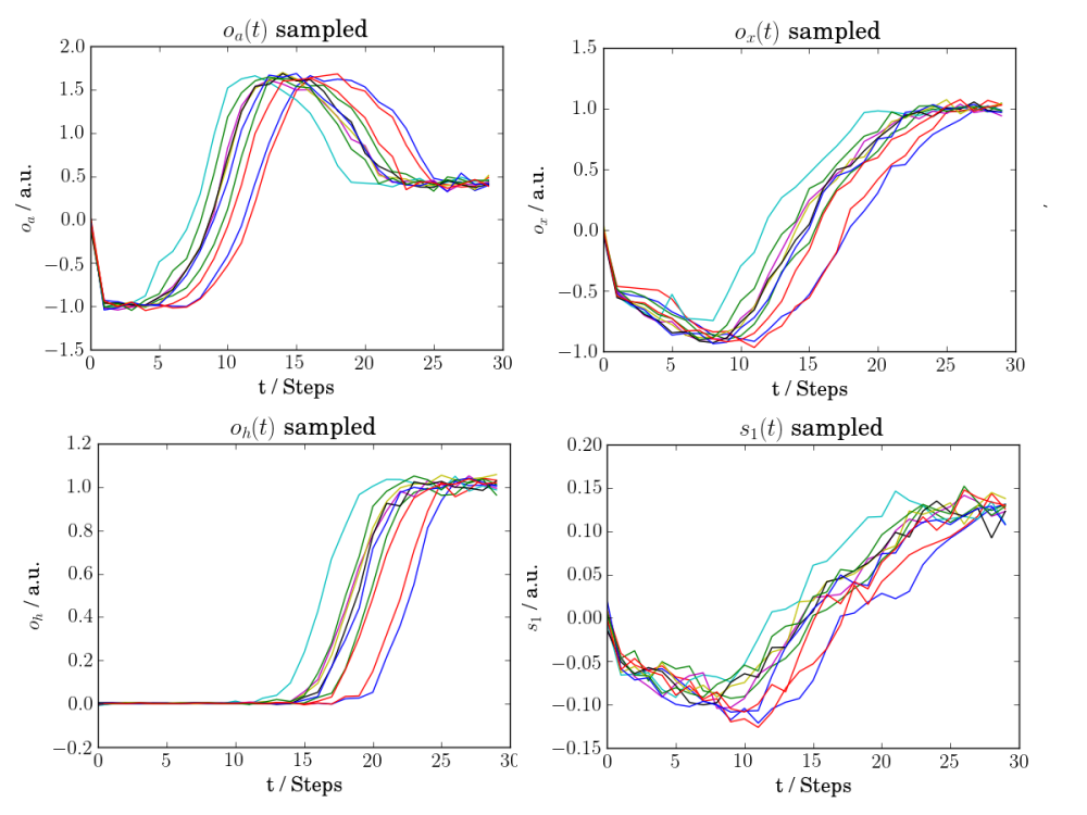 (upper left), the agent’s sense of position (upper right), a nonlinear transformation of the position (lower left), and the agent’s prior expectation on its “homeostatic” state variable (lower right). Note that each distribution is approximated by a single sample per timestep per process.
We see that the agent did not only learn the timecourse of its proprioceptive sensory channel
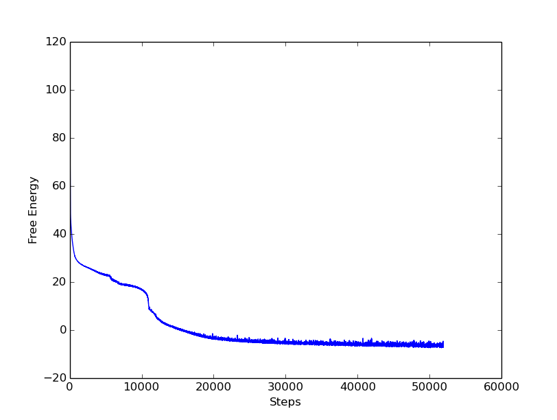
Having such a generative model of the environment, we can not only propagate it freely, but we can also use it to test the hypothesis of the agent, given some a priori assumptions on the timecourse of certain states and/or sensory channels. For this we are using the sampling approach developed in Appendix F of Rezende, Mohamed & Wierstra (and shown in their Figure 5). This way one can for example sample the agent’s prior beliefs about his trajectory 


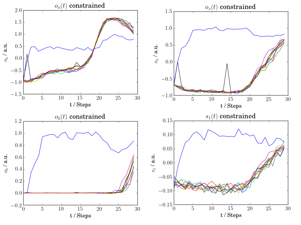 (upper left), using the mean parameters of the population density. Shown are the constrained expectations on the proprioceptive channel (upper left), the agent’s sense of position (upper right), a nonlinear transformation of the position (lower left), and the agent’s constrained expectation on its “homeostatic” state variable (lower right). Note that each distribution is approximated by a single sample per timestep per process.
First, we see that not all of the 10 sampled processes did converge. This might be due to the Markov-Chain-Monte-Carlo-Sampling approach, in which the chain has to be initialized close enough to the solution to guarantee convergence. However, for 9 out of 10 processes, the results look quite reasonable. However, in this example the relative weighting of the agent’s prior expectations on its position is quite strong, leading to the fact that it tightly sticks to the optimal trajectory, as soon as it has learned it. Thus, the dynamics it infers might deviate from the true dynamics. However, if you put the agent in a very noisy environment and take away its effector organs, it reduces to a generative recurrent latent variable model, which has shown to be able to model and generate very complex data.
Outlook
So what are possible directions to go?
First, there are many degrees of freedom in terms of the used nonlinearities, the recurrent architecture of the a priori state transition function, the action function, the variational posterior, or the likelihood functions. So playing with these might actually be very fun and lead to some significant improvements in performance and understanding.
Second, it would be interesting to test this architecture in a more complex setting. A challenging, but realistic next step might be learning pong from pixels and testing the architecture on the Atari 2600 environments.
Third, one could look into implementing more complex a priori beliefs in the model. This could be done by sampling from the agent’s generative model already during the optimisation. E.g. one could sample some processes from the generative model, calculate the quantity on which a constraint in terms of prior expectations of the agent should be placed, and calculate the difference between the sampled and the target distribution, e.g. using the KL-divergence. Then one could add this difference as penalty to the free energy. To enforce this constraint, one could use for example the Basic Differential Multiplier Method (BDMM), which is similar to the use of Lagrange multipliers, but which can be used with gradient descent optimisation schemes. The idea is to add the penalty term 


To optimise the objective 


Fourth, it might be really interesting to see how episodic memory (i.e. an artificial hippocampus) might enhance the agent’s learning, following DeepMind’s cool work on differentiable neural computers.
I think there are even more possible directions to head from here, that’s why I thought it might be nice to put the idea and the code out here and see what people think about it.

Hi Kai, looks very interesting what you wrote here (and also well written) and it is good to see that you could follow a bit more your private endeavour! But I probably have to read it a couple of times more to really get it entirely. I would also love to try out the code. However, I am just using Matlab so far. I am quite sure there a ways around to evaluate Python code in Matlab?! Otherwise, this would be a nice opportunity to learn some Python. 😉
LikeLike
Hi Christoph,
thanks for the nice feedback!
Nevertheless, I will try and clear it up and fix errors as I go along (I’m always thankful for suggestions).
Considering the code: It seems that you can use Python libraries and functions from within MATLAB (https://de.mathworks.com/help/matlab/matlab_external/call-user-defined-custom-module.html) but as far as I understand this also requires you to install Python (https://de.mathworks.com/help/matlab/getting-started-with-python.html). So why not directly install Python and give it a try? Anaconda (https://www.continuum.io/downloads) is a really nice Python distribution. Just make sure to download and install the Python 2 (2.7) version. Then you need to install Theano, which does the heavy lifting in terms of tensor (i.e. high-dimensional “matrix”) operations (and can do so in parallel on the GPU): http://deeplearning.net/software/theano/install.html . If you’re using Ubuntu, you can just follow the instructions here (e.g. under “Stable Installation With conda”): http://deeplearning.net/software/theano/install_ubuntu.html
Cheers,
Kai
LikeLike
Thank you for the helpful tips. Much appreciated!
LikeLike
Hi Kai,
I was just wondering if you have any thoughts on how your work could be applied to mental health epidemiology. So say for example we can observe streams/timer-series of the actions of a population of study participants/agents. To make things simple say that there are three internal latent states, happy, intermediate and depressed. As a psychiatrist we gather observation of say 500 streams of actions over a year. We also gather daily questionnaires which give us a time-series of labels for internal states. I guess then the standard deep learning tool box could be used to fit a recurrent variational auto-encoder onto the time-series of observed actions. And then from the features learnt from this generative model (i.e. using the encoder), we would try to fit a classifier to the labels of the internal states. Thus we have an discriminative model which takes as input sequences of observations of actions, and gives as output classes of internal states.
In this setting the psychiatrist would input new patients observed actions into the trained model to try to infer when a patient is in the intermediate latent state. They could then intervene before they drop into the depressed state.
So basically my question is how could one design a simulation environment, similar to an OpenAI environment to run such a n synthetic experiment, using your framework? It’s not so clear to me how to setup such a three state-switching model?
I was just wondering whether you’ve tried to do this, and what your thoughts might be regarding the simplest way to build such a state space simulator? I’d really like to try this, as it seems like it would give the necessary proof of principle required, before trying to use real epidemiological data.
Best regards,
Ajay
LikeLike
Dear Ajay, thank you for the nice question. To me, your objective sounds more like a classification problem, with the aim of classifying an observed behavior (i.e. series of actions) into three categories (which you derive from the questionnaire data of a training sample). One could first use a variational autoencoder to build a latent representation of the series of actions and train some standard classifier (Support Vector Machines, Random Forests, Supervised Neural Networks) on the autoencoder’s latent representation to predict the true mental state derived from the questionnaires. This should work better than training it on the raw behavioral data directly. However, there is a very nice publication showing how semi-supervised learning (semi-supervised means that you do not even need the actual mental state of every patient/control subject that you use to train your classifier, as it can also use unlabeled data to improve the structure of the latent representation) using deep generative models. I highly recommend this here: https://arxiv.org/abs/1406.5298 This paper works on stationary data, i.e. images for example or time series of fixed length. For action sequences or time series of variable length, it might make sense to extend this framework with a generative *time series* model, i.e. combining this paper with this one: https://arxiv.org/abs/1506.02216 . They both use the same variational formalism, but the latter implements generative models of time series using recurrent neural networks, which allow for a hidden state variable that represents time courses of previously encountered states and actions, i.e. it can be used to compress a long time series of actions into a fixed-size representation. Sorry, the answer got a bit technical but I hope it might help. Cheers, Kai
LikeLike
Hi Kai, indeed as you suggest, the semi-supervised approach is what I’m working on at the moment! The problem of inferring what a study participants “true” mental state is kind of vague – at the moment, questionnaires are what’s used, but the study I’m involved is looking to use wearable devices and smartphone data, to passively get at better measurement of the latent state – if you’re interested check out the major depression study here – https://www.radar-cns.org/major-depressive-disorder.
The three regime/state example I used above is really just a “toy model”. As you said it’s much better to used the latent “features” from a variational-auto-encoder, to “somehow” selct the correct actions of the clinician who want to intervene to help the participant reach a target “high” reward state at the end of the study.
One way maybe of thinking of this is as a problem with sparse rewards, which are only observed at the end of the study. So to make things simple, say we can observe the participants actions only, (but not their latent states), and at the end of the study we simply observe a reward of 1 or -1. So now we want to somehow train a model on this data.
Now using this trained model, we have a new population of patients, and our goal to intervene in their lifestyles, such that we maximize the number of trajectories which finish after some length of time with a +1 reward rather than descending to a terminal reward of -1.
I think for this problem formulation, unsupervised learning, non-differentiable optimization methods (aka evolutionary strategies), and RNNs are the promising “tools”, and I really like your work! I’m not so sure though any of the current DL paradigms can be used “off the shelf” here though? For this particular problem the boundary between the patients actions and the clinicians interventions/actions to steer the trajectory to the +1 terminal reward is not so clear. Also working with historical data rather than a simulator is more challenging. That’s what I like generative unsupervised models, as you can just simulate them forward, and then use black-box optimization to “get the actions”.
Thanks very much for introducing me to the “A Recurrent Latent Variable Model for Sequential Data”, it looks pretty helpful – there’s actually some PyTorch code here – https://github.com/emited/VariationalRecurrentNeuralNetwork – I’ll see whether I can get it working?
Hope this all make sense?
Best,
Ajay
LikeLike
Dear Ajay,
thank you for the clarification and the nice words.
You are right, this sounds more like a reinforcement-learning (RL) problem than a classification problem. However, you are also right, that most Reinforcement Learning approaches (I think even those using those using evolution strategies) might fail without a “simulator” to let the agent explore the environment and how it reacts to different actions. However, I also think that using a Variational Recurrent Neural Network (c.f. Chung et al.) might be a good idea. It can learn a generative model of the time series of all variables that you measure. Later you could just propagate the model, using the variational density q, to encode a given trajectory and then do constrained sampling of the distributions of future timesteps to find out good strategies to improve patients trajectories (c.f. appendix F of Rezende, Mohamed, and Wierstra (https://arxiv.org/abs/1401.4082), algorithm 4 in my deepAI paper, and lines 862ff. of https://github.com/kaiu85/deepAI_paper/blob/master/sample_deepAI_paper.py). This way you could even use standard backpropagation, as in the reference implementation of Chung et al. (https://arxiv.org/abs/1506.02216) to learn a generative time series model and then use constrained sampling to explore how certain actions or other conditions change the trajectory. This is just a rough idea and I might now have it thought trough completely, so take this with care ;o) Otherwise I think this is an awesome area of research and I wish you the best of luck with this project.
Cheers,
Kai
LikeLike
Hi Kai,
thanks for the really nice words and taking the time to write. If you’re interested the pilot project which the major depression study builds on investigated the relationship between sleep, and relapse of negative/depressive symptoms of schizophrenia – here’s a video https://skillsmatter.com/skillscasts/10009-data-vis-in-healthcare (from 4:00 onwards)
Perhaps you might be interested also in some recent work which uses recurrent GANs to simulate real-valued medical data – using the eICU dataset – RGAN – https://arxiv.org/abs/1706.02633. I’m working on tidying up the code for this one, as it could be useful for building a simulator for the data we collect from our patients wearable devices. A similar project which builds a simulator for the frequency of occurrences of diagnostic codes in EHRs is – MedGAN – https://arxiv.org/pdf/1703.06490.pdf. At the moment this one is static, i.e. it doesn’t model the temporal evolution of the entries to the EHRs, but hopefully that will come in the very near future.
So in summary, building a simulator for populations of patients from their EHRs and other electronically harvested data, does seem like a possibility in the future – whether that is accomplished using recurrent GANs or VAEs or VRRNs or something else is still open. The basic idea of a generative recurrent auto-encoder though seems like the right idea, as once trained the decoder can be used as the “simulator”, which could then feed in to the encoder and conditionally on the last periods actions output useful “features” which could then be used to guide clinical decision making in the current period.
I guess until this modelling is done though it’s probably too early to start thinking about RL or other paradigms for automatically recommending psychiatric interventions. It’s a very practical area for ideas from computational psychiatry to develop – but unfortunately many of the academics in the field didn’t seem very interested when I mentioned it at this years London computational psychiatry course? The only lecture that close to what we’ve mentioned above was Chris Mathy’s HGF, but that’s only univariate at the moment, so not really very useful. The data we’ll be harvesting will be high dimensional, highly irregular/mixed frequency and multi-modal. So far I think one of the more promising ways to deal with that “messyness” is by using multi-task Gaussian processes to smooth the data, before sampling from them and passing that regularly structured data into the RNN – a really nice example of a high-dimensional (discriminative) working system which does that is MGP-RNN – https://arxiv.org/abs/1706.04152 – it uses a combination of over 40 different streams, physiological, lab tests, administered medicines,… , to predict the onset of sepsis.
It’s really nice though that you think it’s an interesting area of research as your work seems like it could form a bridge between epidemiological studies, building clinical inference & decision systems for psychiatry, and tests of deep active inference – it’s definitely exciting stuff 🙂
Best wishes,
Ajay
LikeLike
Thank you for the information, right now I’ll really busy but I will look into it! Cheers and all the best, Kai
LikeLike
Hi Kai,
I just thought you’d like to see this by Karl, just in case you’ve not seen it before,
Active Inference, Curiosity and Insight –
Youtube video – https://www.youtube.com/watch?v=Y1egnoCWgUg
Paper – http://www.mitpressjournals.org/doi/abs/10.1162/neco_a_00999
Best wishes,
Ajay
LikeLike
Thank you for the pointer! Karl presented this work during the Computational Psychiatry Course 2016 and I really, really liked it! I just removed a link from your post that might have been a bit problematic due to copyright issues, I hope you don’t mind. Cheers, Kai
LikeLike
Hi Kai,
I’ve read your paper over twice and am excited to try playing with it in Tensorflow. I saw your code on GitHub doesn’t have a license — would you mind adding one? Thanks!
LikeLike
Hi Adam,
thank you for pointing this out. I just added the MIT license to the repository. So have fun!
Cheers,
Kai
LikeLike
Amazing write-up. I have been watching Friston’s lectures online and reading his paper and couldn’t quite get the whole picture. You made it so clear. Thank you!
LikeLiked by 1 person
Thank you! Glad it helped! 🙂
LikeLike
Excellent post and amazing work on this project! I am a PhD student in cognitive neuroscience interested in modeling human behavior (and brain activity) using the free-energy framework. Do you think that it would be reasonable to use something like your deep active inference agent to model human performance in simple sensorimotor tasks? Do you think your agent performs anything like how a human does?
LikeLike
Thank you for the nice feedback. The agent uses some approximations from machine learning, e.g. amortisation, very simple “layers” and stochastic gradient descent based training, about whose physiological plausibility one could argue. Furthermore, it has no really intermediate stochastic representations, but only a single latent space. To be honest, to model sensorimotor decision tasks, maybe a model closer to physiology might be more useful, e.g. in terms of drift diffusion models, which can be generalised to multiple choices and which can be derived from noisy attractor models of decision making (https://journals.plos.org/ploscompbiol/article?id=10.1371/journal.pcbi.1000046, https://www.biorxiv.org/content/10.1101/542431v1, https://www.ncbi.nlm.nih.gov/pubmed/12467598). Alternatively you might look into more biologically grounded implementations of active inference/predictive coding. Personally, I’ve never worked with this, but there have been some great recent works using the hierarchical gaussian filter to fit individual behavior (https://www.ncbi.nlm.nih.gov/pubmed/28798131, https://www.frontiersin.org/articles/10.3389/fnhum.2014.00825/full).
LikeLike
Hi, Kai, amazing work! I’m trying to get your code to run, but having some difficulty. Do you plan to port it to python 3?
LikeLike
Hi, Jordan.
Thank you for the kind words.
Please forgive the enormous delay. Currently, I have to work full time in a surgical department as part of my final months in med school. After that, there are serious plans to port the code to Python3 and PyTorch (and plans for some exciting extensions, I‘ve started three drafts before the clinical work swamped me).
Cheers,
Kai
LikeLike